内容
图像处理课程第二次作业
1. Questions
1.1
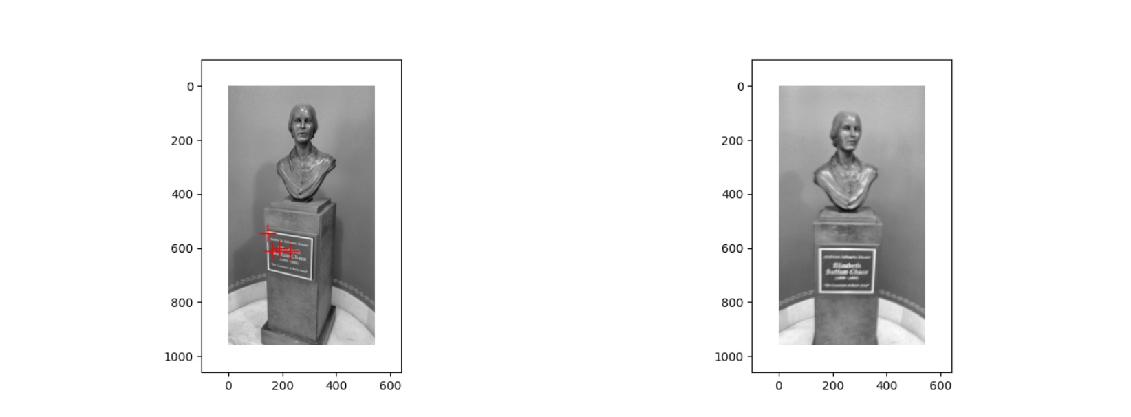
上面是第一对图片经过 Harris corner detection 得到的结果,可以看到第一张图片有四个角点,而第二张图片一个都没有,从原图以及结果来看,出现这种情况的原因应该是第二张图片的清晰度比较低,比较模糊,因此在各个位置的 cornerness score 会比较低,没有超过 Threshold,所以没有检测出角点
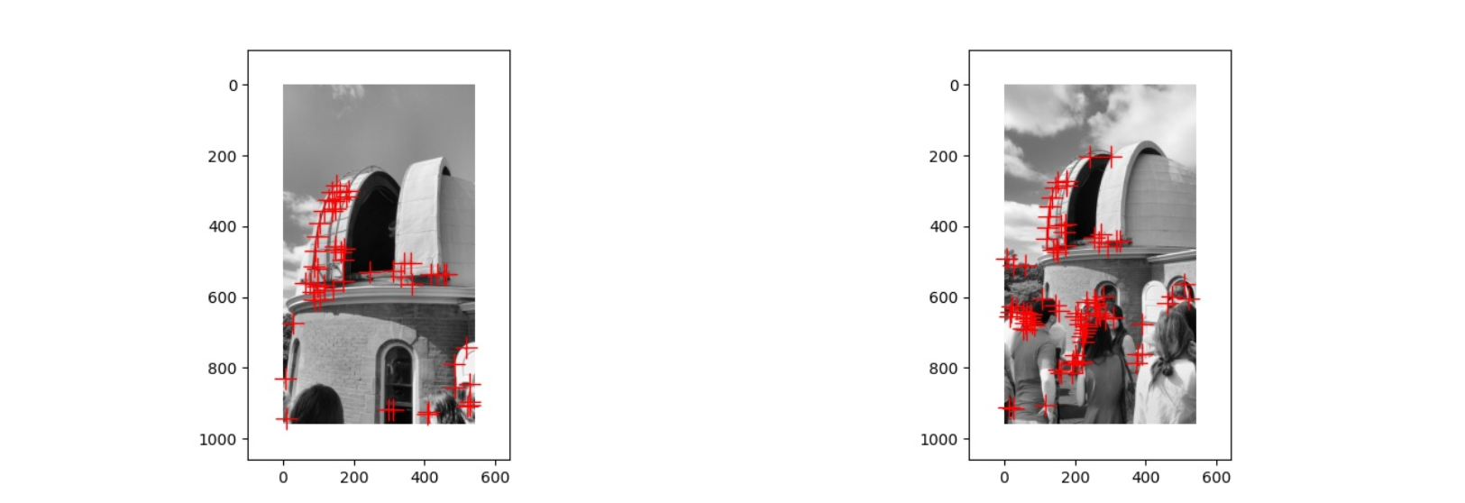
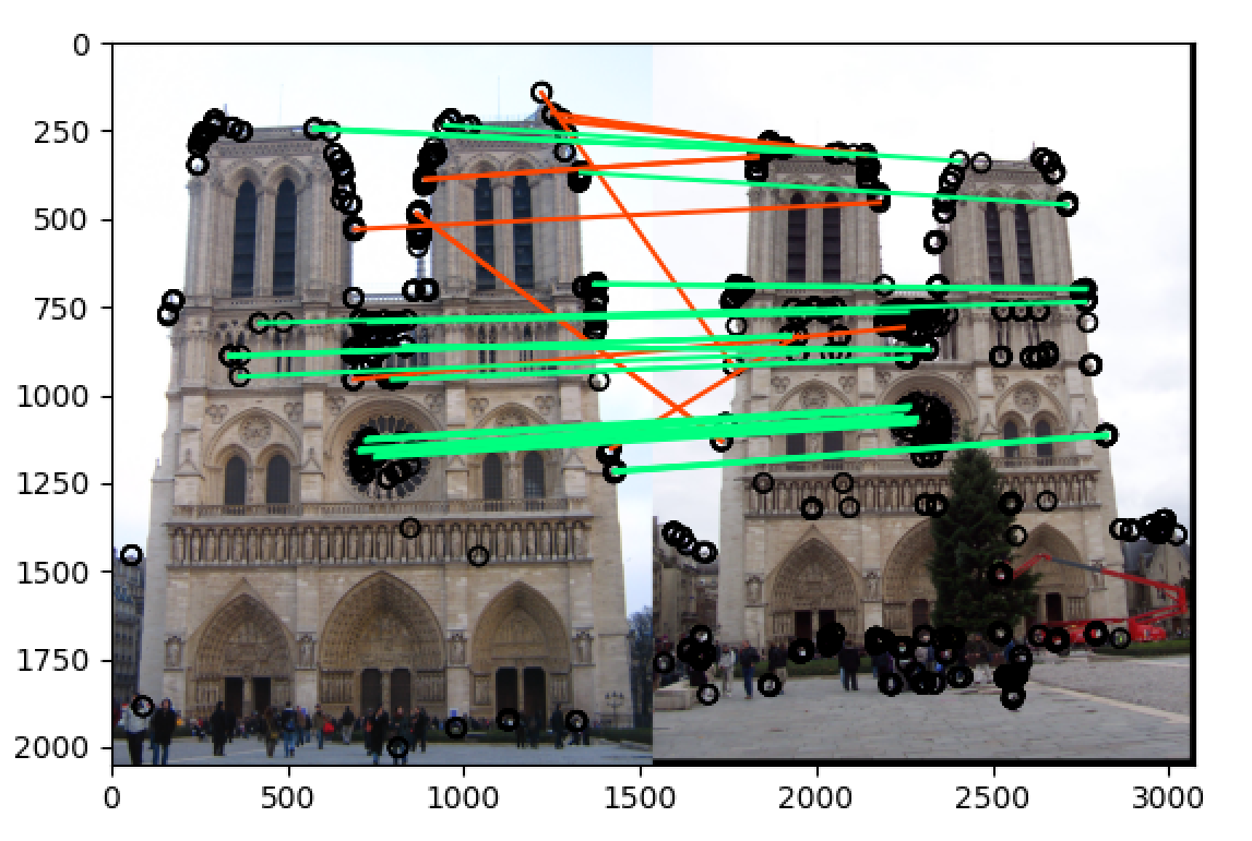
上面是第二对图片经过 Harris corner detection 得到的结果,与第一张图片相比,第二张图片中建筑的拍摄角度不太相同,并且还有许多其他的人或景物,因此位于建筑上的角点比较少,而且还有很多位于其他地方的角点,出现这种情况就是因为拍摄的角度问题,以及其他人和景物的干扰
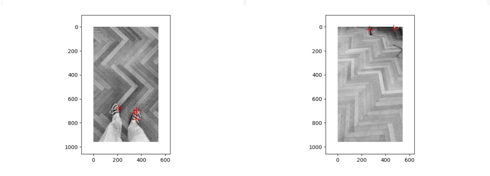
上面是第三对图片经过 Harris corner detection 得到的结果,第一张图片中的角点都集中在鞋子上,第二张图片中的角点都集中在边缘的一些椅子腿之类的东西上面,而两张图片在地板上都没有出现角点,出现这种情况的原因可能是地板的特征值变化不大,没有超过 Threshold,因此角点都在其他的物体上
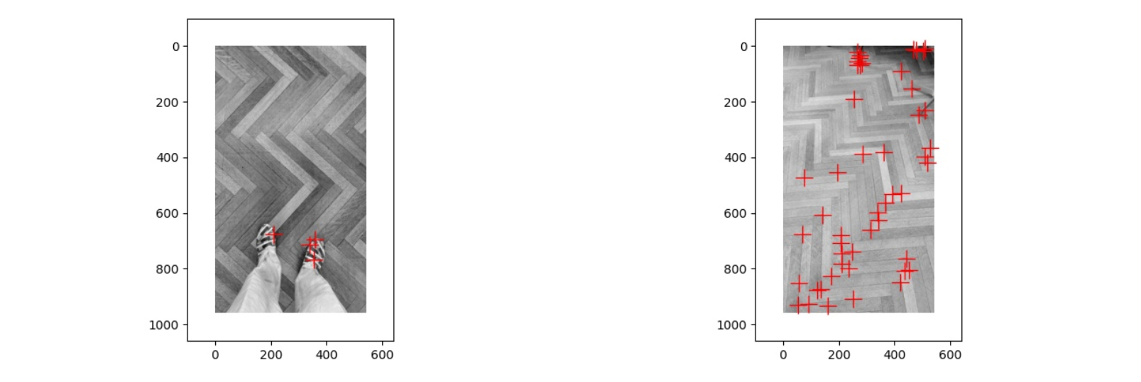
于是我将 Threshold 从 0.5 改为了 0.01,在这种情况下第一张图片的角点不变,而第二张图片中出现了很多,这种情况下两张图片的不同就是由于光线的区别
因此在现实世界中,无论是拍摄的清晰度,拍摄的角度,其他物体的干扰,以及拍摄时的光线,滤镜等,都会对于图片的特征匹配造成影响,而同时代码中对于 threshold 或是其他参数的设置,也会有一定的影响
1.2
local image brightness 在哪个方向变化的越快,那么那个方向的特征值就会越大
我们可以将M可视化为椭圆,其轴长由M的特征值决定,方向由M的特征向量确定
1.3
1 | # You can assume access to the image , x and y gradients , and their magnitudes / |
1.4
(a) 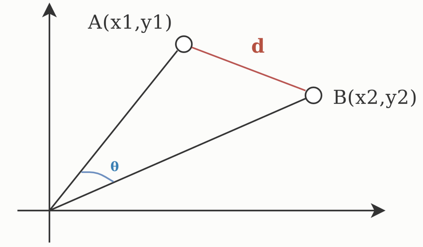
如图是两个向量 A(x1, y1) 和 B(x2, y2),那么欧氏距离就是两个向量之间的实际距离 d,而余弦相似度为两个向量之间的夹角 θ,因此当向量的大小无关紧要时,余弦相似度通常用作距离的度量,而当向量的大小重要的时候需要使用欧氏距离作为距离的度量
(b) 如果给定了一个距离度量的方法,我们可以使用 Nearest Neighbor Distance Ratio 的方法来进行特征匹配,对于第一幅图中的每个点,计算出第二幅图中与其最近的距离和第二近的距离的比例,将所有点的比例按照从小到大排序,即为匹配的准确性的排序,因为这个比例越大,就代表第二幅图中有其他点与要匹配的点的相似度越高,那么进行特征匹配的准确率就越低,而比例越小,就代表这个点越独特,也能更好的作为要匹配的特征点
1.5
(a)
line 是由满足坐标 (u+λa, v+λb), ∀λ ∈ R 的点组成的,对于其中的每一个点 (x, y),经过变换后的点满足
因此变换后的线是由满足坐标
的点组成的
(b)
要使变换后的线汇聚到一个点,那么对于任意的 λ ,坐标都应该是一样的,那么有以下几种情况:
a=0, b=0 此时汇聚点的坐标为
a=0, H 的第二列均为0 此时汇聚点的坐标为
b=0, H 的第一列均为0 此时汇聚点的坐标为
H 的第一列和第二列均为0 此时汇聚点的坐标为
(c)
如果 a, b, H的第一列的值, H的第二列的值不满足上一问的任何一种情况,则变换后的线不会汇聚到一个点
2. Programming Project
2.1 Implement match_features()
计算欧氏距离
1 | dist = [] |
开始写了一个循环版本的,后来看到要求使用 numpy 中的函数不能用循环,就写了一个计算欧氏距离的函数
1 | def euclidean_distances(a, b): |
要求 a,b 两个集合中的元素两两间欧氏距离,先求出 a 乘 b 的转置,然后对 a 和 bt 分别求其中每个向量的模平方,并使用 tile 函数扩展为原来的大小,然后相加减去 2倍 的 a 乘 b 转置开平方就得到了结果,开平方之前把小于零的变为0,防止开平方出错
最近邻匹配
1 | matches = np.zeros((len(im1_features), 2)) |
对于第一幅图片的每一个特征点,在第二幅图片中找到欧氏距离最小的点作为匹配点,计算最小的距离和第二小的距离的比,将这个比的倒数作为 confidence
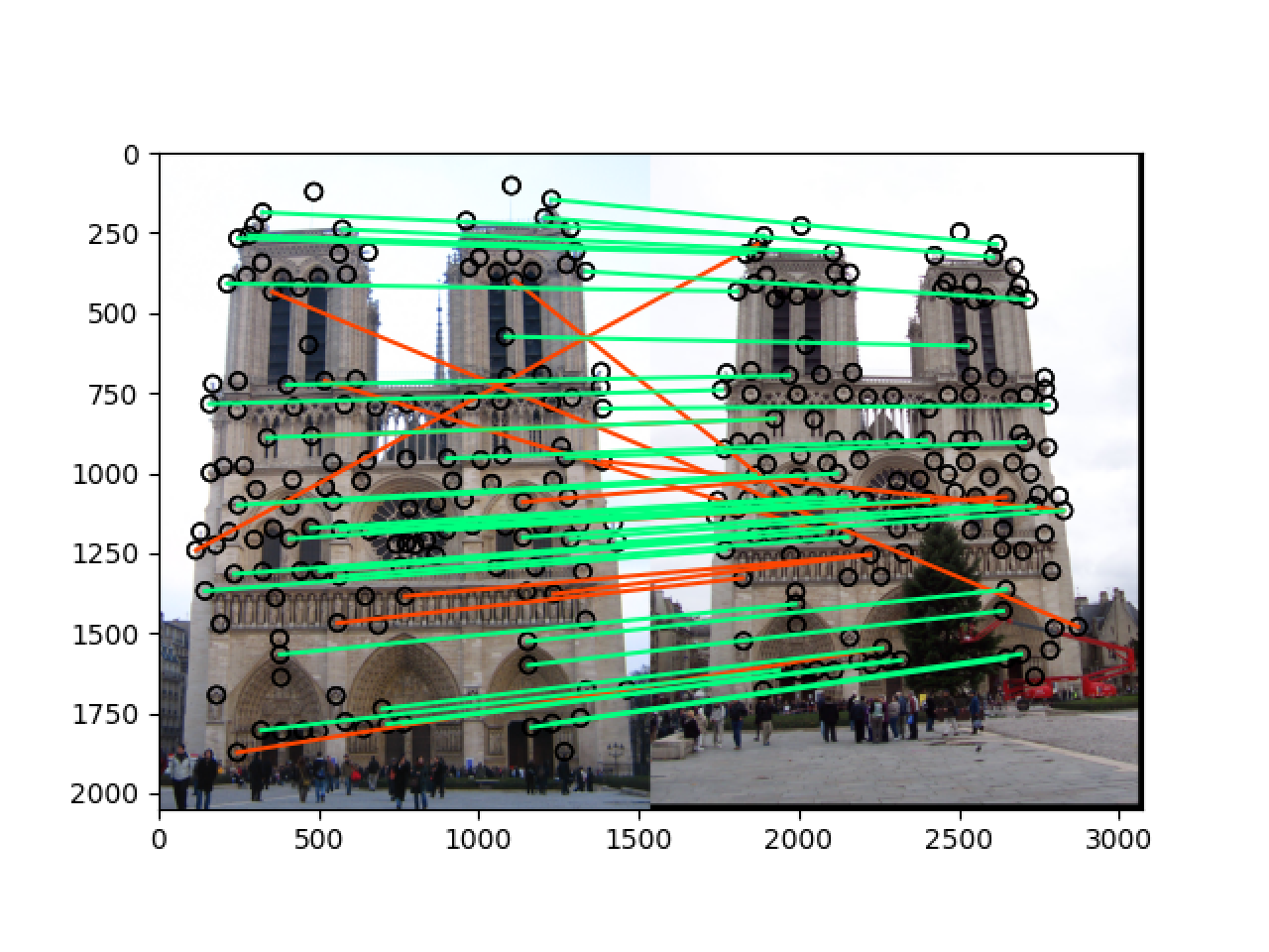
此时在总共149个匹配中只有一个能匹配成功
2.2 Change get_features()
1 | features = np.zeros((len(x), 256)) |
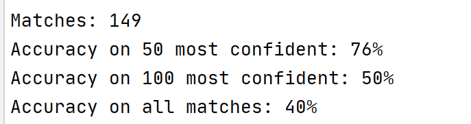
直接使用 image 里面的值作为特征值,此时的结果为:
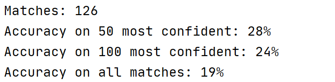
2.3 Finish get_features() by implementing a SIFT-like feature
1 | features = np.zeros((len(x), 128)) |
对于每一个关键点,将以关键点为中心的 feature_widthfeature_width 大小的区域划分为 `44=16个小区域,计算出每一个区域在八个方向上的梯度大小,拼接成长度为448=128` 的特征向量,最后进行归一化,此时结果如下: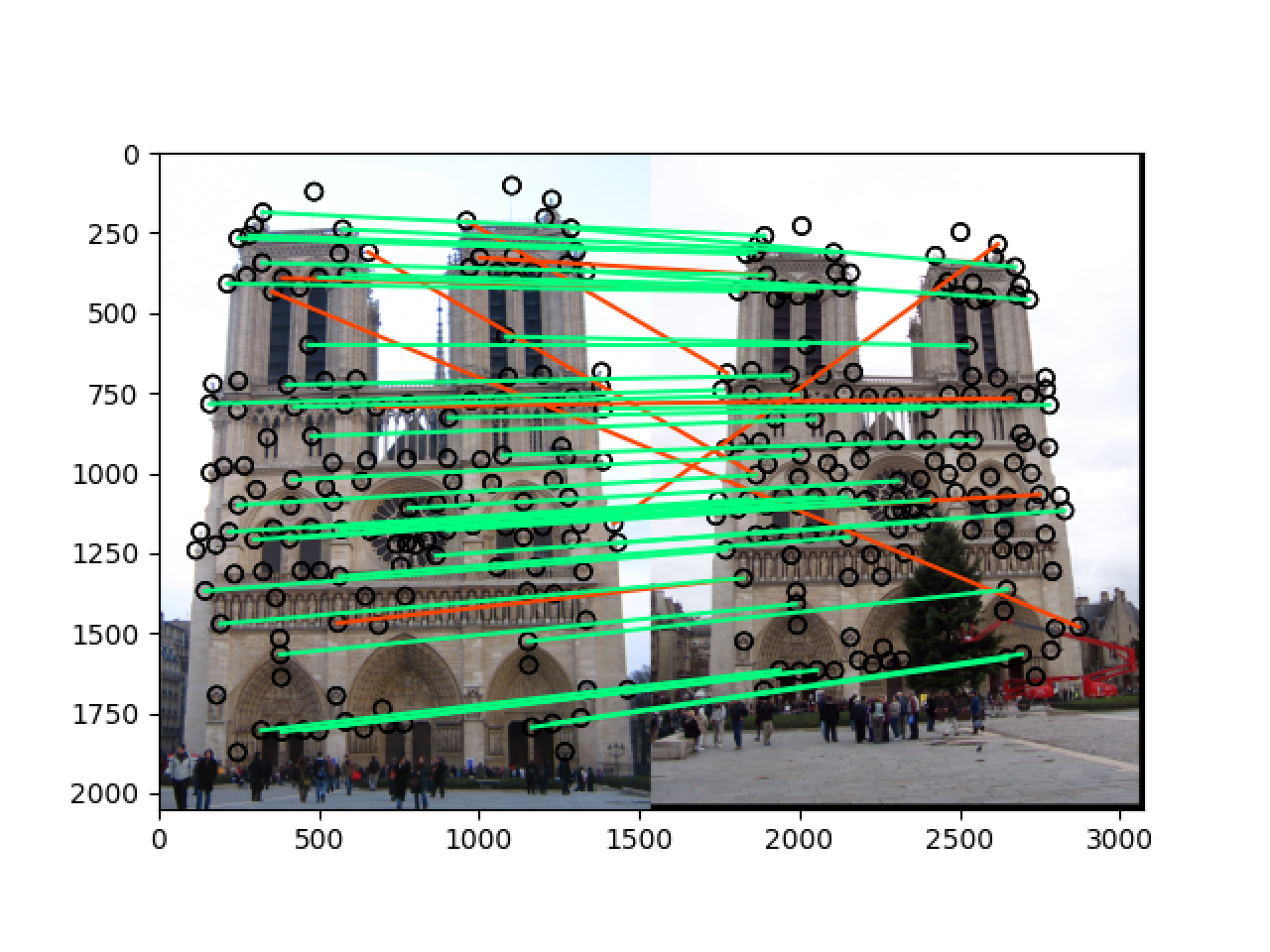
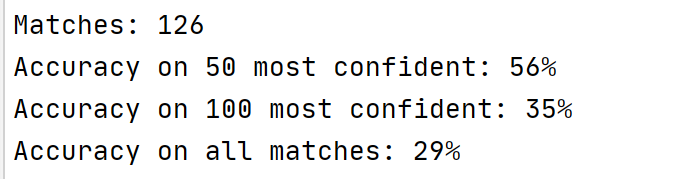
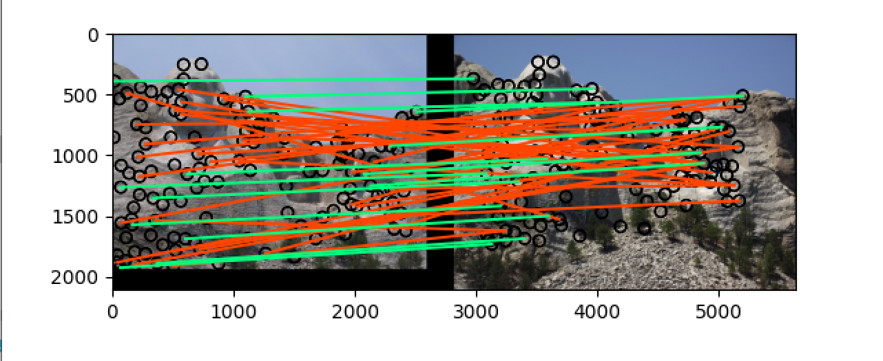
可以看到准确率在 notre_dame 上提升了一点,但是在 mt_rushmore 上提升了许多
2.4 Stop cheating and implement get_interest_points()
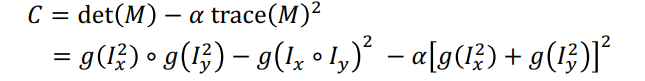
在开始的时候我没有在多尺度上提取关键点,只是使用了 Harris Corner detection,首先对输入的图片进行一次高斯滤波,高斯核大小为
3*3,sigma为1,随后对处理之后的图片计算出 x 方向和 y 方向的梯度grad_x和 grad_y,随后计算出grad_x*grad_x,grad_x*grad_y,grad_y*grad_y, 再对这三个梯度分别进行一次高斯滤波,高斯核大小为9*9,sigma为2,然后利用下面的公式计算出每个点的 cornerness,为了避免边缘效应,我将图片 feature_width 大小的边缘的值设置为0,随后先利用 threshold 得到 cornerness 较大的点,再使用 cv2 中的 dilate 将每个点的值变为局部极大值,然后得到这些局部极大值对应的点,即为我们要寻找的关键点,但是这样测试的结果不太稳定,即准确率随 threshold 值的变化而产生的变化很大因为我看到实验结果不是很好,所以紧接着就决定在多个尺度上进行特征提取
$\textcolor{red}{Extra\ credit} $:Detect keypoints at multiple scales
在多尺度上检测关键点就是建立高斯金字塔和差分金字塔,其中多尺度指的是对同一幅图片用不同的高斯核进行滤波,来得到图片的不同尺度的特征,然后寻找特征点的时候要判断特征点的 cornerness 值是否在差分金字塔的当前尺度和相邻尺度的邻域最大,然后据我调查,高斯金字塔设置为多个组的原因是工程上的需要,因此我在本次实验中只计算并使用了和输入图片相同大小的一个组。
具体代码如下:
1 | start = time.time() |
- 根据输入图片用不同的高斯核向同组的上一张图片进行滤波,得到高斯金字塔的一个组 octave
- 计算出差分金字塔
- 对于差分金字塔的每一层,像原来一样计算出梯度,进行高斯滤波,计算每一个点的 cornerness 值,去除边缘效应,其中我将阈值 threshold 设置为 cornerness 的最大值除以十,因为不同的图片所需要的阈值不同,因此这样设置能得到相对还可以的关键点的数量,在除以十的情况下,image1中得到的关键点的数量和题目中提到的300~700相一致,然后用dilate在当前尺度下进行膨胀操作
- 因为我们要求的关键点不仅要在当前尺度局部最大,还要在相邻尺度局部最大,因此我们在另一个维度也进行膨胀操作,随后得到局部极大值的坐标和对应尺度并返回
$\textcolor{red}{Extra\ credit} $:Multi-scale descriptor
既然我们已经在多个尺度上提取了图像的关键点,那么在提取特征的时候也要从对应的尺度来提取,因此要对原有的代码进行更改,首先就是在函数开始用和上面同样的方法计算出相应的高斯金字塔和差分金字塔,在提取特征的时候,先根据特征的尺度确定要在哪张图片上提取特征,随后跟之前一样提取一个128维的特征即可
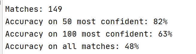
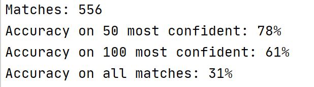
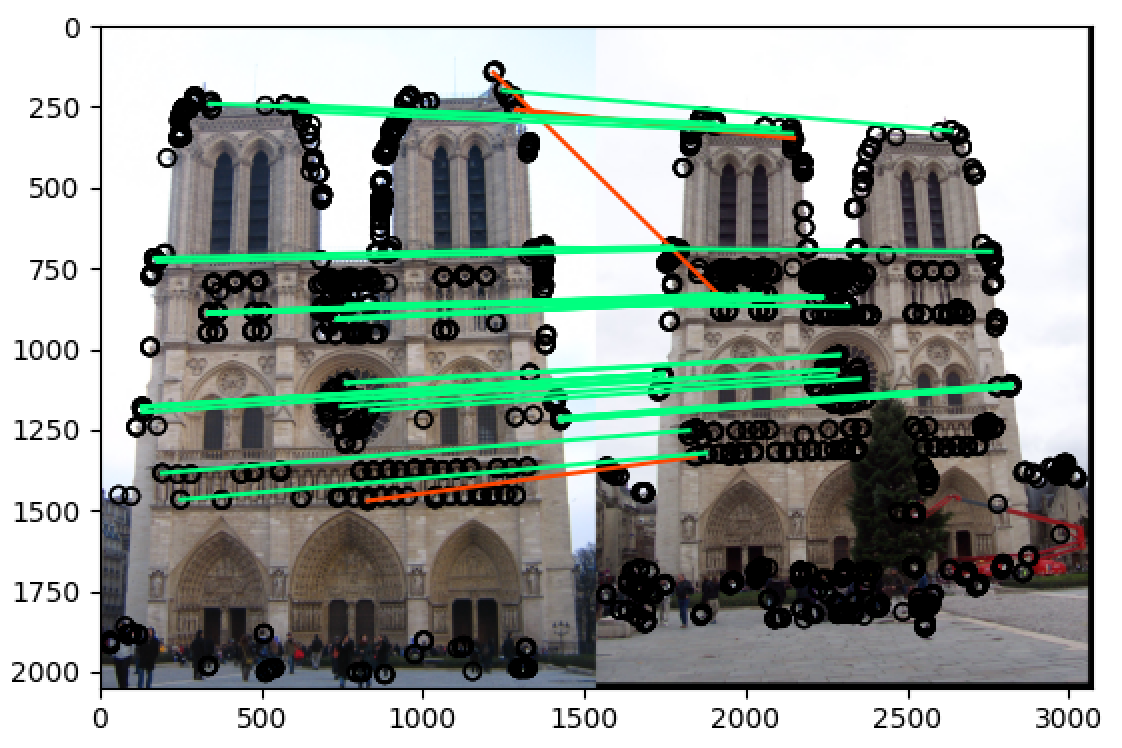
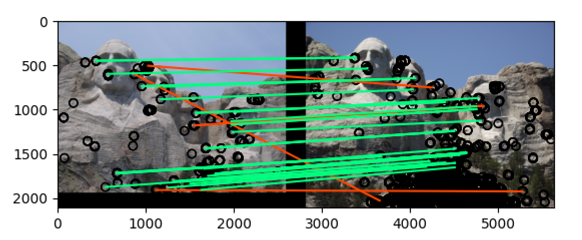
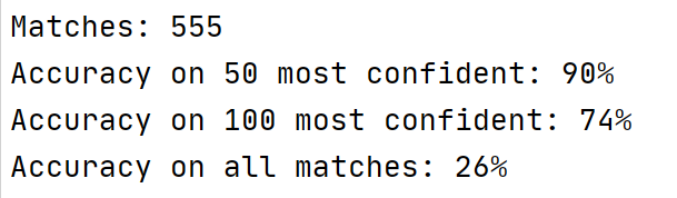
最终结果
notre_dame
将 threshold 改为 最大值除以20:t = np.max(h)/20
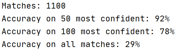
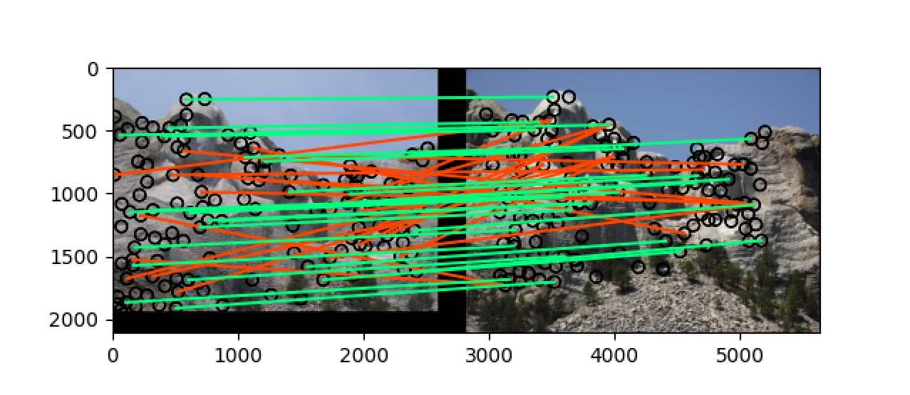
mt_rushmore
将 threshold 改为 最大值除以20:t = np.max(h)/20
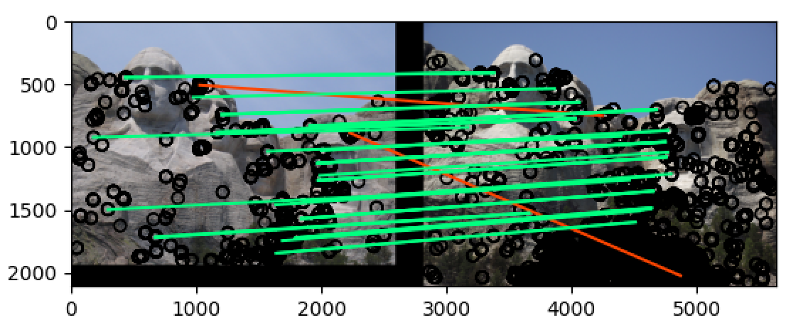
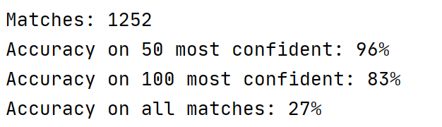
可以看到最终再 notre_dame 和 mt_rushmore 两组图片中的准确率都非常高,当
t = np.max(h)/10的时候,notre_dame 在 50 most confident 的匹配准确率为 78%,而 mt_rushmore 在 50 most confident 的匹配准确率为 90%,而当t = np.max(h)/20的时候,两组图片在 50 most confident 的匹配准确率都达到了 90% 以上,即使是在 100 most confident 中也分别达到了 70%+ 和 80%+ 的准确率,远远高于题目中的要求